Scipy stats

Contents

• Scipy stats
  • Setup
  • The Kolmogorov-Smirnov test
  • A Chi-square approach

Scipy contains a library with statistical functions, distributions and tests, called scipy.stats. In this example, we will explore some of the possibilities it offers, tackling the following problem from asteroseismology of sdB stars (see e.g. Kawaler 1988):

Due to the interior structure of an sdB star, we expect long pulsation periods to follow an equidistant pattern (i.e., a period spacing). The value of the period spacing tells us more about the extent of the core and the envelope.

A complication is that often, not only periods from a period spacing are observed, but also other frequencies, e.g. due to rotational splitting. So given a list of observed periods, we need to find the value of the period spacing, and perhaps test whether it is significant.

We use two approaches to this problem:

• Following Kawaler 1988, we perform the Kolmogorov-Smirnov test to see whether a certain period spacing is significant. Doing this for a lot of trial period spacings, we can make some kind of periodogram.
• We run over a grid of possible periods, and compute the chi-square statistic for every trial period (and offset).

The second strategy is incredibly crude, and, scientifically, not really the way to go. However, it allows us to use the chi-square distribution implemented in scipy to derive confidence intervals on the period spacing (and offset).

Setup

To explore this problem, we will simulate an observed set of period spacings, and add some noise to them.

First, we need to do the usual imports:

import numpy as np
import pylab as plt
from numpy import pi
import scipy.stats

Now, generate 8 almost equidistant spacings, and add 3 random ones periods mixed with the equidistant structure. We fix the seed to be able to reproduce the results:

np.random.seed(1111)
periods = 1.23 + np.arange(8)*0.43 # the spacing and offset
periods += scipy.stats.norm.rvs(size=len(periods),scale=0.005) # add normal noise
periods = np.hstack([periods,scipy.stats.uniform.rvs(size=3,loc=1.23,scale=3)]) # mix with 3 others
periods.sort()

Note that we could have used the np.random module too to generate the random variables. However, the scipy.stats module contains much more distributions and many more options. For every statistical distribution, you can

• generate random variables with .rvs()
• compute the probability density function with .pdf()
• compute the cumulative density function with .cdf()
• ... and much more

This is a list of spacings we want to test:

test_spacings = np.linspace(0.05,1,1000)

The Kolmogorov-Smirnov test

The following few lines of codes closely follow Kawaler (1988). Since this is not a tutorial on statistics, we refer to that paper for more information.

We choose the shortest period to compare with, and remove it from the list of periods.

index_short = np.argmin(periods)
p_short = periods[index_short]
periods_del = np.delete(periods,index_short)

Then, we calculate the distribution of the periods compared to the tested spacing:

dp = []
for dp_test in test_spacings:
    ri = []
    for pi in periods_del:
        ni = (pi-p_short)/dp_test
        ri.append(ni-np.floor(ni))
    dp.append(ri)

Next, we use the Kolmogorov-Smirnov test to derive whether the ri come from a uniform distribution. We do this for every test spacing:

Q = np.zeros(len(dp))
for i,ri in enumerate(dp):
    ksstat,pvalue = scipy.stats.kstest(ri,'uniform')
    Q[i] = pvalue # we're only interested in the pvalue, not the KS statistic

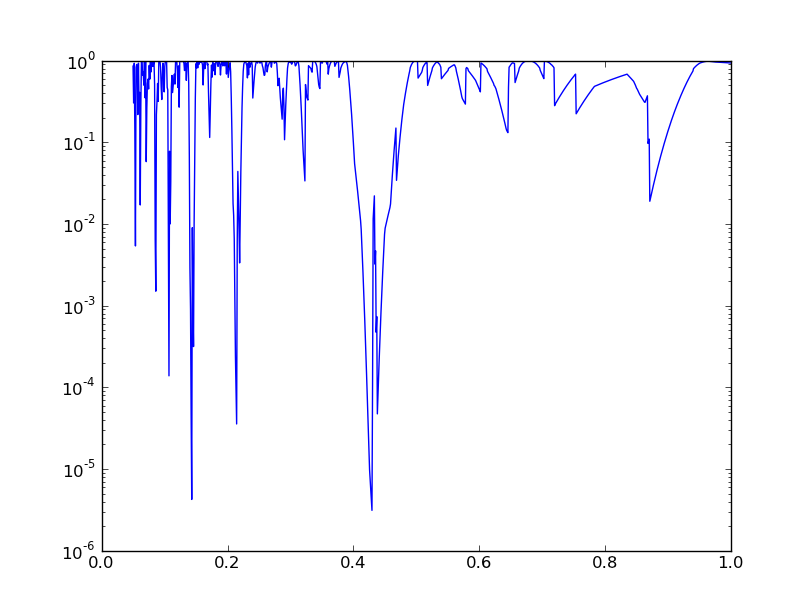
In principle, we should now correct for the number of trial periods (the Bonferroni correction, but we omit that step here. Finally, we can make a plot:

plt.figure()
plt.plot(test_spacings,Q)
test_spacings[np.argmin(Q)]

A Chi-square approach

The chi-square approach requires us to check a set of predicted period spacings, which all have their own offset value and period spacing, against the observed set of period spacing. We will make the huge assumption that we already know that we have 8 periods within a period spacing.

We have to cycle over all the possibilities, build the set of period spacing, and match them with the closest values in the set of observed periods (we do not care about the three random ones, but we do not know which ones the are).

Let us first make a search grid:

test_offset = np.linspace(1.2,1.25,500)
test_spacings = np.linspace(0.3,0.5,500)

And prepare for the computation of the chi-square statistic. We have 8 periods to match and free parameters, so we need to set k=8-2=6 in the chi-square distribution:

chi2 = np.zeros((len(test_offset),len(test_spacings)))
k = 8-2

Next, we run over the grid and compute the chi-square statistic, which is defined as the sum of the residuals-squared divided by the error-squared:

for i,to in enumerate(test_offset):
    for j,ts in enumerate(test_spacings):
        test_periods = to+np.arange(8)*ts
        periods_ = periods[:-1] + np.diff(periods)/2.
        closest_index = np.searchsorted(periods_,test_periods)
        chi2[i,j] = np.sum((periods[closest_index]-test_periods)**2/0.005**2)

Using scipy.stats, we can compute the cumulative density of the chi-square value, which corresponds to some kind of confidence rating:

chi2_stat = scipy.stats.distributions.chi2.cdf(chi2,k)

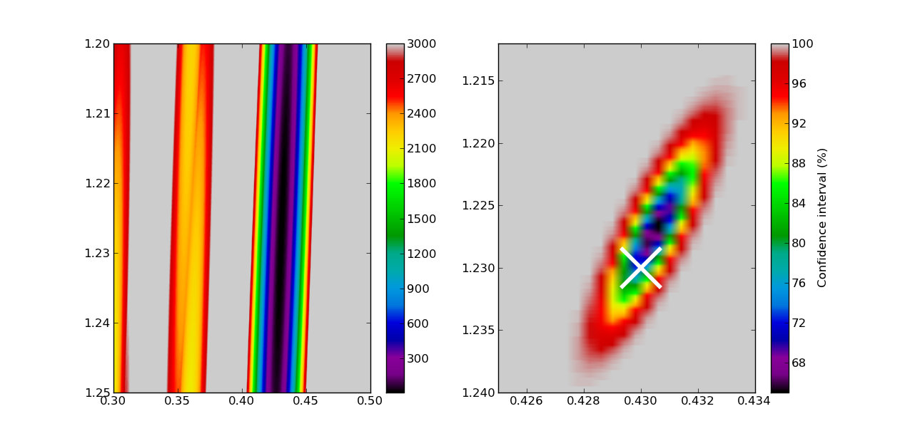
That’s it! All is left is to make some plots: we choose to make a plot of the chi-square values themselves (left), and a plot of the confidence intervals (right).

plt.figure()
plt.subplot(121)
extent = test_spacings.min(),test_spacings.max(),test_offset.max(),test_offset.min()
plt.imshow(chi2,aspect='auto',extent=extent,vmin=10,vmax=3000,cmap=plt.cm.spectral)
plt.colorbar()
plt.subplot(122)
plt.imshow(chi2_stat*100,aspect='auto',extent=extent,cmap=plt.cm.spectral)
plt.plot(0.43,1.23,'x',ms=40,mew=4,color='1')
plt.xlim(0.425,0.434)
plt.ylim(1.24,1.212)
cbar = plt.colorbar()
cbar.set_label('Confidence interval (%)')