Scipy FFT

Contents

• Scipy FFT
  • Getting started
  • The analytical broadening kernel
  • The synthetic line
  • The analytical Fourier transform
  • Computing the Fourier transform
  • Measuring the vsini

In this tutorial, we dig a bit deeper in scipy’s 1D FFT capabilities, exploring rotational broadening in stellar spectra along the way. For a full list of available functions, see http://docs.scipy.org/doc/scipy/reference/fftpack.html.

The flow of the programming is as follows (see, e.g., Carroll 1933, Dravins 1990, Reiners 2001, Simon-Diaz 2006):

1. First, we construct a rotational broadening kernel assuming a linear limb-darkened star
2. We generate a synthetic spectral line, and convolve it with the kernel using fftconvolve.
3. We add some noise on the spectrum.

Next, we assume we don’t know the projected equatorial velocity, and derive it from the generated spectrum, using the Fourier method. We compare an oversampled computed Fourier transform (fft) with the analytical one. So the steps are:

4. Compute the fft of the generated spectrum and compare with the analytical one (of the broadening kernel only)
5. Compare the output vsini with input value.

Getting started

We need a lot of functions. First, we import the Fourier functions:

from scipy.fftpack import fft,fftfreq
from scipy.signal import fftconvolve

For the analytical computation of the Fourier transformation, Bessel functions are required:

from scipy.special import j1

And of course the usual imports. An explicit import of pi, sin, cos and sqrt is done to avoid extensive use of np. which could make the code less readable.

import pylab as plt
import numpy as np
from numpy import pi,sin,cos,sqrt

To finalize the setup, we need some constants. We define them here explicitly, but there exists a module scipy.constants, with an extensive list of physical constants. However, it does not contain specifical astronomical constants such as the solar mass (see Prsa & Harmanec 2011).

midwave = 4480. # central wavelength of line
cc = 2.99792458e+18 # velocity of light in angstrom/s
epsilon = 0.6 # linear limbdarkening parameter
vsini = 75.*1e13 # input vsini in A/s (75 km/s)
dlam = 0.01 # spectrum resolution (A)
delta = midwave*vsini/cc

We will add some noise to a generate spectrum. To be able to reproduce the results, we make sure that we always add the same noise, regardless of how many times we run the script:

np.random.seed(1111)

The analytical broadening kernel

The rotational broadening function G is only defined on a certain wavelength interval, but we’ll be lazy and solve that issue later. For now, we make the wavelength interval broad enough, i.e. +/- 5 angstrom, using the spectral resolution given above.

lambdas = np.linspace(-5,5,10./dlam+1) # wavelength interval
y = 1-(lambdas/delta)**2 # transformation of wavelengths
G = (2*(1-epsilon)*sqrt(y)+pi*epsilon/2.*y)/(pi*delta*(1-epsilon/3))  # the kernel
print(G)

The sqrt is of course only defined for positive numbers. For negative numbers, numpy silently fills in nan (not a number).

Click to Show/Hide: NOTES on ``np.nan``

Note

• in some versions of scipy and numpy, nan is not silently introduced, but a warning is printed to the screen. You can avoid these print statements via np.seterr(all='ignore').

• In the example, we were lazy and let the nan be introduced in the arrays. In general, you should be very careful with this behaviour, since many statements will silently break if there are nan’s around:

  x = np.random.normal(size=100)
  x.std()
  x[10] = np.nan
  np.std(x) # std is not defined when there is a nan!
  

  Some functions have an alternative that can handle nans:

  np.nanmax(x)
  

  but not all of them:

  hasattr(np,'nanstd'), hasattr(np,'nansum')
  

• You might think np.nan is a good way to mask elements in an array, e.g. when you want to compute the mean of an array. However, in the previous note we’ve seen that numpy functions will return np.nan when used on an array containing at least on np.nan. Numpy has a seperate array class for arrays with masked values, appropriately named masked arrays:

  x = np.random.normal(size=(4,4))
  x
  mask = x<0
  y = np.ma.array(x,mask=mask)
  y
  

  Notice that numpy actually uses a specific fill value for the masked values, usually 1e+20, but you can control that value. Then finally, we can use the normal numpy functions again:

  x.std(),y.std()
  x.min(),y.min()
  

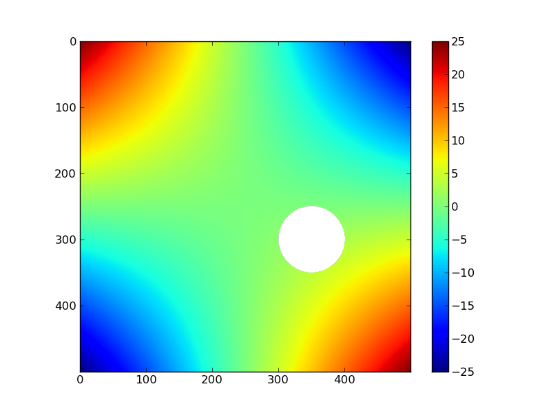
• matplotlib can handle np.nan:

  X,Y = np.mgrid[-5:5:500j,-5:5:500j]
  Z = X*Y
  Z[np.sqrt((X-1)**2+(Y-2)**2)<1.] = np.nan
  plt.imshow(Z);
  plt.colorbar();
  

We remove all the wavelength and kernel elements wherever the kernel is not defined:

keep = -np.isnan(G) # returns boolean array with `False` where there are nans
lambdas,G = lambdas[keep],G[keep] # crop the arrays not to contain nans
lambdas.min(),lambdas.max()

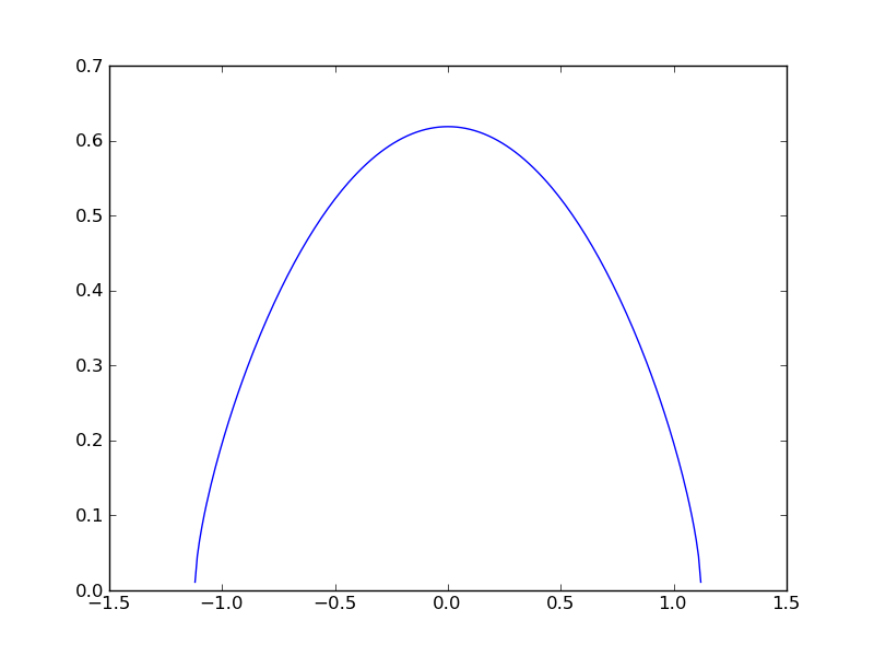
The broadening kernel is only defined between -1.12 and 1.12 A. We could have foreseen this, since

1.12/midwave*(3e5) # approximate velocity in km/s of 1.12 angstrom at 4480A

Finally make a plot of the rotational kernel.

plt.plot(lambdas,G)

The synthetic line

Suppose a line has an intrinsic Gaussian profile in absence of rotation:

wavelengths = np.arange(midwave-5,midwave+5+dlam,dlam)
spec_line = 1-0.5*np.exp( -(wavelengths-midwave)**2/(2*0.1**2)) # width of 0.1A

This needs to be convolved with the rotational broadening kernel. Scipy (and numpy) have a convolve function that does not use the FFT, but here we choose to use the FFT version. We construct the new wavelength array for the convolved spectrum, and make sure the equivalent width has not changed during the convolution process:

spec_conv = fftconvolve(1-spec_line,G,mode='full')
N = len(spec_conv) # equals len(spec_line)+len(G)+1 when mode='full'
wavelengths_conv = np.arange(-N/2,N/2,1)*dlam + midwave
EW_before = np.trapz(1-spec_line,x=wavelengths) # trapezoidal integration
EW_after = np.trapz(spec_conv,x=wavelengths_conv)
spec_conv = 1-spec_conv/EW_after*EW_before

Click to Show/Hide: NOTE on numerical integration

Note

Scipy contains a package dedicated to integration: scipy.integrate. It also contains the trapz function, implements the Simpson rule, and provides quad and dblquad, that can integrate functions numerically between limits (i.e., without you having to specify an x and y array):

In [1]: from scipy.integrate import quad

In [1]: quad(lambda t: np.exp(-t) / t**5,1,np.inf)
Out[1]: (0.0704542374617277, 2.8164841189102693e-09)

The return value is a tuple, with the first element holding the estimated value of the integral and the second element holding an upper bound on the error.

The integrate package also contains an ODE solver odeint. See e.g. the Zombie Apocalypse example.

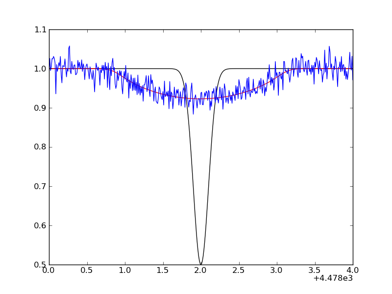
Finally, we simulate an observed profile by adding random Gaussian noise:

spec_obs = spec_conv + np.random.normal(size=len(spec_conv),scale=0.02)

A plot of the unbroadened (black) and broadened line (red/blue) can be made with:

The analytical Fourier transform

Let’s get back to the rotational kernel. The analytical Fourier transform is easily computed. First, we need to define the domain in frequency space on which to compute the transform, and then we evaluate it. Note the use of scipy’s Bessel function:

x = np.linspace(0,30,1000)[1:]  # exclude zero
g = 2. / (x*(1-epsilon/3.)) * ( (1-epsilon)*j1(x) +  epsilon* (sin(x)/x**2 - cos(x)/x))
g = g**2 # convert to power

x /= (2*pi*delta)

Computing the Fourier transform

When calculating the FFT with fft, a complex array is returned. You can get the real and imaginary part with y.real and y.imag, and the norm and phase angle via np.abs(y) and np.angle(y). In this case, we are only interested in the power. Also, we need to increase the frequency resolution of the Fourier transform, so that we can nicely resolve the zeros. This is done via zero padding, and there exists and optional keyword n to the function fft to do just that. If you do not specify n, n equals the length of the input array, otherwise the input array is zero-padded until it is of size n. We choose to make our input array 100 times larger. Finally, the Fourier method is sensitive to noise outside of the spectral line region. Therefore, we cut the spectrum to have little continuum remaining.

keep = np.abs(midwave-wavelengths_conv)<1.2 # minimize contribution of continuum
spec_to_transform = (1-spec_obs)[keep] # we need the continuum at zero
new_n = 100*len(spec_to_transform) # new length for zeropadding
spec_fft = np.abs(fft(spec_to_transform,n=new_n))**2 # power of FFT

The domain of the Fourier transform is retrieved via fftfreq, but we exclude the negative frequencies:

x_fft = fftfreq(len(spec_fft),d=dlam)
keep = x_fft>=0 # only positive frequencies
x_fft, spec_fft = x_fft[keep], spec_fft[keep]

Measuring the vsini

The measured vsini corresponds to the first zero in the Fourier transform. Due to discretization and noise, zero will never be reached, so we need to look for local minima: those are the locations where the first derivative switches sign from negative to positive:

neg_to_pos = (np.diff(spec_fft[:-1])<=0) & (np.diff(spec_fft[1:])>=0)
minima = x_fft[1:-1][neg_to_pos]

Let’s compare that to the minima from the analytical transform:

neg_to_pos = (np.diff(g[:-1])<=0) & (np.diff(g[1:])>=0)
minima_an = x[1:-1][neg_to_pos]

The frequency domain can be converted to velocity (km/s) as follows:

q1 = 0.610 + 0.062*epsilon + 0.027*epsilon**2 + 0.012*epsilon**3 + 0.004*epsilon**4
vsini_zeros = cc/midwave*q1/minima/1e13
vsini_zeros_an = cc/midwave*q1/minima_an/1e13

The first zero should be the input vsini:

print(vsini_zeros_an[:10])
print(vsini_zeros[:10])

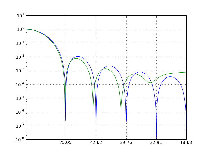
Finally, we can make a nice plot: We use the s/A scaling on the x-axis, but set the tickmarks to correspond to km/s.

plt.figure();
plt.plot(x,g/g.max());
plt.plot(x_fft,spec_fft/spec_fft.max());
plt.gca().set_yscale('log');
plt.xlim(0.0,0.05);
plt.ylim(1e-8,1e1);
plt.grid();
plt.xticks(minima_an[:5]*midwave/q1/cc*1e13,['{0:.2f}'.format(i) for i in vsini_zeros_an[:5]])