Standard Python Tools
There are two standard “core” Python modules that provide much of the functionality necessary to access internet resources from inside python: urllib2 and urllib. You have seen urllib2 in each of the prior workshops when downloading example files or datasets, like this:
import urllib2
url = 'http://python4astronomers.github.com/_downloads/image_sources.csv'
open('image_sources.csv', 'wb').write(urllib2.urlopen(url).read())
Webpage Retrieval
It is useful to write the example above a bit differently since readability counts and we want to highlight a few steps:
handler = urllib2.urlopen(url)
data = handler.read()
handler.close()
f = open('image_sources.csv','wb')
f.write(data)
f.close()
First, urllib2 has returned a file like object handler that points to a specific web resource. Various attributes about the webpage are available:
print handler.code
print handler.headers['content-type']
In this particular example the data request is handled after the initial response has been examined; the data is streamed into a local variable data and then saved to a local file. As demonstrated in the asciitable portion of the Reading and Writing Files workshop, one alternatively could parse the returned data stream into a table for further use.
Building Queries
Now we are getting closer to searching for data online via python. Traditionally, each data archive has implemented its own set of query parameters; more often than not you experience it as a web form with lots of check and input boxes. Most of the time these web forms are simply input wrappers that build a query string and process the result.
Here is a very simple query example: search for HST images near M 51. It is worth noting that you have to find and read the MAST HST documentation to learn which parameters are needed to build the query:
import urllib2, urllib

# this is the query url for this service.
url = 'http://archive.stsci.edu/hst/search.php'

# make a dictionary of search parameters
p = {}
p['target']="M 51"
p['radius']=1.0
p['max_records']=10
p['outputformat']='CSV'
p['action']='Search'

# encode the http string
query = urllib.urlencode(p)

# create the full URL for a GET query
get_url = url + "?" + query

# create the GET handler
handler = urllib2.urlopen(get_url)

# check it
print handler.code
print handler.headers['content-type']

# save it
f = open('hst_m51.csv','wb')
f.write(handler.read())
f.close()
The magic is that urllib module takes care of encoding the parameters using standard HTTP rules. You can compare the input dictionary key,value pairs with the HTTP url encoding:
# some simple formatting where the format %-M.Ns means
# "-" :: 'left justified'
# "M" :: 'minimum string length, padded'
# "N" :: 'maximum string length, sequence sliced'
# "s" :: 'format as string'
sform = "%-20.20s %-10.10s %-30.30s"

# make a header
print sform % ('parameter', 'value', 'encoded')
print sform % (3 * (100 * '-',))

# for each parameter show the input items from the dictionary
# "p" and the output query string.
for a,b in zip(p.items(), query.split('&')):
   print sform % (a + (b,))
Exercise: import WISE catalog data for a young cluster
In this exercise you will use a different service (IRSA) and with a different overall goal for these data:
import atpy, urllib, urllib2

url = "http://irsa.ipac.caltech.edu/cgi-bin/Gator/nph-query"
p = {}
p['spatial'] = "Cone"
p['objstr'] = "IC 348"
p['outfmt'] = 1    # IPAC table format
p['catalog'] = 'wise_prelim_p3as_psd'
p['radius'] = 300

query = urllib.urlencode(p)
get_url = url + "?" + query
handler = urllib2.urlopen(get_url)
raw = handler.read()
print raw[0:255]

f = open('ic348_wise.tbl', 'wb')
f.write(raw)
f.close()
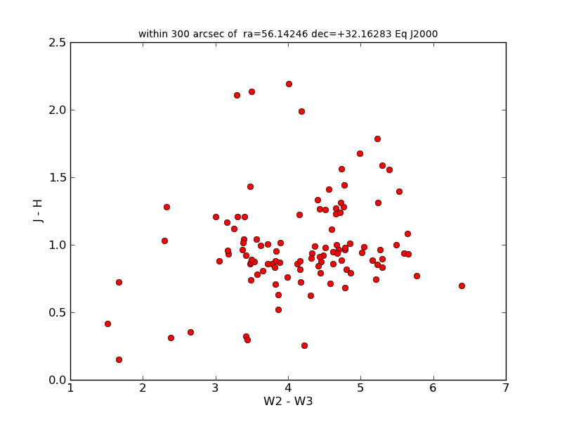
The challenge is to immediately analyze the results of this query. The exercise is to make a simple color-color plot of these objects.
Click to Show/Hide Solution
There are several ways we have looked at in the workshops for converting this result to a numpy array. We’re going to use atpy to read in the table:
t = atpy.Table('ic348_wise.tbl')
You’ll notice that atpy automatically detects that this in ipac table, and automatically replaced ‘null’ values with nan, correctly converts all the data types, and preserves more of the metadata of the query. Now we can make a quick plot that reuses some of this metadata in the plot title:
plt.clf()
plt.plot(t['w2mag'] - t['w3mag'], t['j_m_2mass'] - t['h_m_2mass'], 'ro')
plt.xlabel('W2 - W3')
plt.ylabel('J - H')
plt.title(t.keywords['SKYAREA'], fontsize='small')

Read the instructions!
Because these web interfaces vary from archive to archive it is worth emphasizing that building the query string for a particular data archive begins with reading the documentation page for that archive’s GET interface.
Here are some links to these documentation pages for some archives
and the service url for these are:
