1D Examples and Exercise

Here we will run over a few simple examples using the curve_fit function for fitting data similar to emission and absorption spectra. We will not use any real data here, but simulate simple data to see how well we can fit the data.

Simple Gaussian

Let’s begin with a simple Gaussian problem. We will generate fake data first and compare it to the real data:

import numpy as np
from scipy.optimize import curve_fit
import matplotlib.pyplot as mpl

# Let's create a function to model and create data
def func(x, a, x0, sigma):
    return a*np.exp(-(x-x0)**2/(2*sigma**2))

# Generating clean data
x = np.linspace(0, 10, 100)
y = func(x, 1, 5, 2)

# Adding noise to the data
yn = y + 0.2 * np.random.normal(size=len(x))

# Plot out the current state of the data and model
fig = mpl.figure()
ax = fig.add_subplot(111)
ax.plot(x, y, c='k', label='Function')
ax.scatter(x, yn)
fig.savefig('model_and_noise.png')

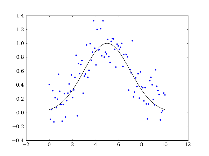
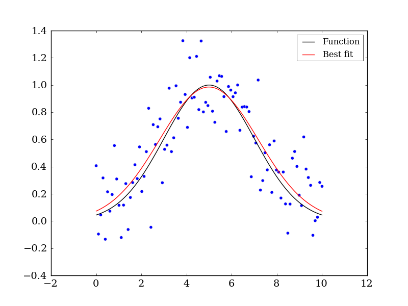
Let’s now use curve_fit function to see how well we can reconstruct the the data’s original form before noise was added:

# Executing curve_fit on noisy data
popt, pcov = curve_fit(func, x, yn)

#popt returns the best fit values for parameters of the given model (func)
print popt

ym = func(x, popt[0], popt[1], popt[2])
ax.plot(x, ym, c='r', label='Best fit')
ax.legend()
fig.savefig('model_fit.png')

Multiple Gaussian

The optimization function curve_fit seems quite simple to use. When using it with simple and clean situations as shown above it can excel quite nicely. But, what about when there’s multiple Gaussian peaks and dips (i.e. emission and absorption) in a dataset?:

import numpy as np
from scipy.optimize import curve_fit
import matplotlib.pyplot as mpl

# Let's create a function to model and create data
def func(x, a, x0, sigma):
    return a*np.exp(-(x-x0)**2/(2*sigma**2))

# Generating clean data
x = np.linspace(0, 20, 200)
y1 = func(x[np.where(x <= 10)], 1, 3, 1)
y2 = func(x[np.where(x > 10)], -2, 15, 0.5)

y = np.hstack([y1, y2])

# Adding noise to the data
yn = y + 0.2 * np.random.normal(size=len(x))

# Plot out the current state of the data and model
fig = mpl.figure()
ax = fig.add_subplot(111)
ax.plot(x, y, c='k', label='Function')
ax.scatter(x, yn)
fig.savefig('model_and_noise_multiple.png')

# Executing curve_fit on noisy data
popt, pcov = curve_fit(func, x, yn)

#popt returns the best fit values for parameters of the given model (func)
print popt

ym = func(x, popt[0], popt[1], popt[2])
ax.plot(x, ym, c='r', label='Best fit')
ax.legend()
fig.savefig('model_fit_multiple.png')

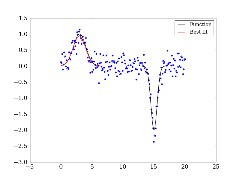
Exercise 1

Using the code from above utilize the help or ? functionality in ipython to figure out how fit the dip. Otherwise, you can always refer to the online documentation for curve_fit.

to reproduce (within reason) the image below. Additionally, using the tabbing feature to see what other methods are available is key for this exercise. Use the Quick Reference Guide for other information that may be helpful.

Click to Show/Hide Hint

It’s all about the initial parameters.

Click to Show/Hide Solution

Use the optional parameter p0 for the initial conditions:

popt, pcov = curve_fit(func, x, yn, p0=[-1,15,1])

The next obvious choice from here are 2D fittings, but it goes beyond the time and expertise at this level of Python development. If you do need such a tool for your work, you can grab a very good 2D Gaussian fitting program (pure Python) from here. For high multi-dimensional fittings, using MCMC methods is a good way to go. One of the simplest and fastest MCMC packages is emcee.